Analysis: The ASTI Intensity Index

Data

• Procedures and Definitions
• Financial Years
• Adjusting Expenditures for Inflation
• Purchasing Power Parity Exchange Rates
• Cost Categories
• Funding Sources
• Full-Time Equivalents (FTEs)
  

Analysis

• ASTI intensity index
• R&D investment and knowledge stocks
• TFP projections

Practitioner's guide

Practitioner's guide for national and regional focal points (PDF)

Sample surveys

ASTI’s primary data surveys differ according to the type of agencies being surveyed. The following are downloadable examples of ASTI’s surveys in Excel format:

• Government and nonprofit agencies
• Higher education agencies
• Private, for-profit companies

The ASTI Intensity Index

The data envelopment analysis (DEA) approach is used to obtain the ASTI Intensity Index (AII) and to calculate feasible levels of investment and investment gaps for individual countries. The AII calculates the R&D investment intensity of a country relative to the main structural factors affecting intensity: the size of the agricultural sector (proxied by AgGDP), the size of the economy (proxied by GDP), income (proxied by GDP per capita), and potential spill-ins (proxied for a country i as the sum of R&D investment of all other countries weighted by a measure of the similarity of country i’s output composition with output composition of each other country). These four variables are proxies for structural variables that constraint policymakers’ decisions on R&D. For example, R&D investment in a low income country with a small economy would probably invest proportionally less in R&D than a high income country with a large economy because of a small market for innovation and constrained supply of researchers due to a less developed education system, quality of research institutions and budget constraints among several other factors.

In generic form, this measure can be represented as:

\( AII_{i} = f[{({R\&D_{i}}\over{GDP_{i}})},{({R\&D_{i}}\over{AgGDP_{i}})},{({R\&D_{i}}\over{y_{i}})},{({R\&D_{i}}\over{SP_{i}})}] \) (A.1)

where AIIi is the AII of country i, R&D is expenditure in agricultural R&D, y is income per capita, SP measures potential spill-ins, and f[●] is a function aggregating the four partial intensity measures into a single number that measures the R&D investment intensity of country i. The DEA method looks for endogenous weights to aggregate the partial indices into the overall AII. This approach has been extended more recently to build indices that comply with characteristics required by index theory. The approach used by Whittaker and colleagues (2015) is adapted here to build a multifactored measure of R&D intensity.

The figure below presents in graphic form the main concepts behind the calculation of the index. The axes in the figure represent values of R&D investment relative to two variables, income (GDP per capita) and AgGDP. The use of two inputs in the figure is only for illustrative purposes. Each point in the figure represents a country with coordinates AgGDP/R&D and income/R&D, in the vertical and horizontal axes, respectively. Note that these coordinates represent the inverse of partial intensity ratios, with the measure in the vertical axis being the inverse of the Intensity Ratio normally used to measure the intensity of agricultural R&D investment. The further a country is from the origin, the lower its R&D intensity.

In the case of country D, a valid comparison to determine R&D intensity is to compare it with point D*. This is because D and D* have the same proportion of AgGDP and income (they are in the same ray through the origin). In this case, D* shows much higher values of R&D/AgGDP and R&D/income than D, which means that the R&D intensity of point D* is higher than that of D. Countries A, B, and C in the figure are the countries with highest R&D intensity because there is no other country closer to the origin along the respective rays through the origin than these three countries (rays OA, OB and OC in the figure, respectively).

Investments by countries A, B, and C outline the “intensity frontier.” This frontier defines the space of investment intensity for the sample of countries, with the highest intensity defined by points A, B, and C, and by all linear combinations of these three points (the lines connecting A, B, and C). Countries with less intensive investment are in the space above and to the right of the frontier. How do we calculate the distance of country D to the frontier? For example, the intensity measure for country D can be calculated as AII_D = OD*/OD, which is the distance of country D to the frontier. This distance is a measure of the difference of investment intensity between D and the maximum potential investment (investment at the frontier). Countries at the frontier also have, by definition, intensity index values equal to 1 because the distance of each of these countries from the frontier is AII_A = OA/O_A = AII_B = OB/OB = AII_C = OC/OC = 1. Countries in the intensity space above the frontier will show AII values between 0 and 1. Comparing frontier countries with country D in the figure establishes the intensity indexes AII_A = AII_B = AII_C = 1 ≥ AII_D ≥ 0. The closer the AII is to 1, the higher the investment intensity of that country—that is, the higher R&D investment relative to the value of AgGDP and income.

The discussion on the intuition of the methodology used here shows that the DEA approach allows us to determine the maximum potential intensity that a country can reach (given observed intensities of all countries). As a corollary of this, it allows us to obtain the actual intensity gap for that country, which can be measured as the difference between maximum potential intensity and actual intensity. This method also allows us to express the potential intensity for each country in terms of any of the partial intensity ratios of the AII. For example, as discussed above, the coordinates of the efficient point D* are (AgGDP/R&D)_D*= (AgGDP/R&D)_D×(OD*/OD) and (income/R&D)_D*= (income/R&D)_D×(OD*/OD). From these expressions, we obtain the potential IR for country D as IRP_D=1/[(AgGDP/R&D)_D×(OD*/OD)], as one of the coordinates of the reference point for D at the intensity frontier.

Figure—R&D intensity index using two partial measures of intensity

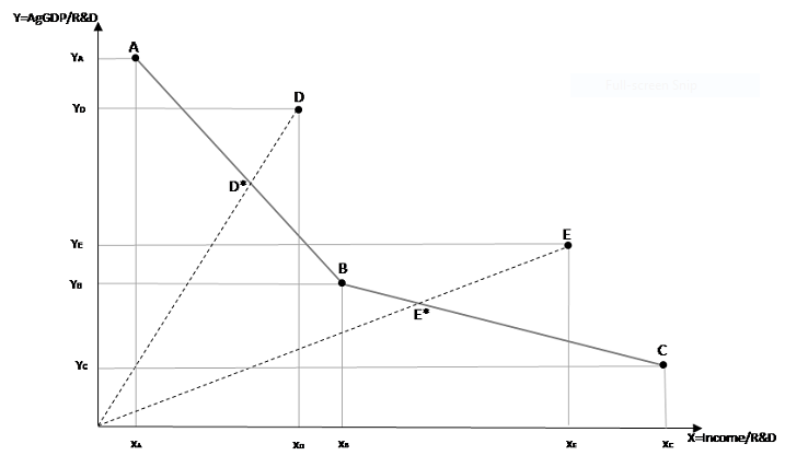
Notes: The intensity ratios are expressed as the inverse of R&D spending / AgGDP and R&D/income, where A, B, and C determine the “frontier”, showing the value of AgGDP and income per unit of R&D invested. AgGDP = agricultural gross domestic product; R&D = research and development.